The portion of the Nyquist plot for gain \(\Lambda=4.75\) that is closest to the negative \(\operatorname{Re}[O L F R F]\) axis is shown on Figure \(\PageIndex{5}\). This is a diagram in the \(s\)-plane where we put a small cross at each pole and a small circle at each zero. Z ( That is, we consider clockwise encirclements to be positive and counterclockwise encirclements to be negative. ) WebNyquist criterion or Nyquist stability criterion is a graphical method which is utilized for finding the stability of a closed-loop control system i.e., the one with a feedback loop. ) must be equal to the number of open-loop poles in the RHP. {\displaystyle 1+G(s)} Looking at Equation 12.3.2, there are two possible sources of poles for \(G_{CL}\). T We know from Figure \(\PageIndex{3}\) that the closed-loop system with \(\Lambda = 18.5\) is stable, albeit weakly. Its system function is given by Black's formula, \[G_{CL} (s) = \dfrac{G(s)}{1 + kG(s)},\]. by Cauchy's argument principle. WebThe reason we use the Nyquist Stability Criterion is that it gives use information about the relative stability of a system and gives us clues as to how to make a system more stable. ( Natural Language; Math Input; Extended Keyboard Examples Upload Random. plane, encompassing but not passing through any number of zeros and poles of a function s We will look a little more closely at such systems when we study the Laplace transform in the next topic. While Nyquist is one of the most general stability tests, it is still restricted to linear time-invariant (LTI) systems. ) While Nyquist is one of the most general stability tests, it is still restricted to linear, time-invariant (LTI) systems. The system is called unstable if any poles are in the right half-plane, i.e. The MATLAB commands follow that calculate [from Equations 17.1.7 and 17.1.12] and plot these cases of open-loop frequency-response function, and the resulting Nyquist diagram (after additional editing): >> olfrf01=wb./(j*w.*(j*w+coj). \[G_{CL} (s) = \dfrac{1/(s + a)}{1 + 1/(s + a)} = \dfrac{1}{s + a + 1}.\], This has a pole at \(s = -a - 1\), so it's stable if \(a > -1\). Note that \(\gamma_R\) is traversed in the \(clockwise\) direction. We draw the following conclusions from the discussions above of Figures \(\PageIndex{3}\) through \(\PageIndex{6}\), relative to an uncommon system with an open-loop transfer function such as Equation \(\ref{eqn:17.18}\): Conclusion 2. regarding phase margin is a form of the Nyquist stability criterion, a form that is pertinent to systems such as that of Equation \(\ref{eqn:17.18}\); it is not the most general form of the criterion, but it suffices for the scope of this introductory textbook. T We consider a system whose transfer function is Its image under \(kG(s)\) will trace out the Nyquis plot. {\displaystyle F(s)} is the number of poles of the open-loop transfer function ( WebFor a given sampling rate (samples per second), the Nyquist frequency (cycles per second), is the frequency whose cycle-length (or period) is twice the interval between samples, thus 0.5 cycle/sample. are also said to be the roots of the characteristic equation 0 {\displaystyle u(s)=D(s)} nyquist stability criterion calculator. For these values of \(k\), \(G_{CL}\) is unstable. charles city death notices. {\displaystyle G(s)} The Nyquist criterion is a graphical technique for telling whether an unstable linear time invariant system can be stabilized using a negative feedback loop. , as evaluated above, is equal to0. ) The system or transfer function determines the frequency response of a system, which can be visualized using Bode Plots and Nyquist Plots. The other phase crossover, at \(-4.9254+j 0\) (beyond the range of Figure \(\PageIndex{5}\)), might be the appropriate point for calculation of gain margin, since it at least indicates instability, \(\mathrm{GM}_{4.75}=1 / 4.9254=0.20303=-13.85\) dB. are called the zeros of The right hand graph is the Nyquist plot. , which is to say our Nyquist plot. s  1 Let us complete this study by computing \(\operatorname{OLFRF}(\omega)\) and displaying it on Nyquist plots for the value corresponding to the transition from instability back to stability on Figure \(\PageIndex{3}\), which we denote as \(\Lambda_{n s 2} \approx 15\), and for a slightly higher value, \(\Lambda=18.5\), for which the closed-loop system is stable. ( My query is that by any chance is it possible to use this tool offline (without connecting to the internet) or is there any offline version of these tools or any android apps. = Suppose \(G(s) = \dfrac{s + 1}{s - 1}\). {\displaystyle N} To connect this to 18.03: if the system is modeled by a differential equation, the modes correspond to the homogeneous solutions \(y(t) = e^{st}\), where \(s\) is a root of the characteristic equation. u = H Refresh the page, to put the zero and poles back to their original state. Section 17.1 describes how the stability margins of gain (GM) and phase (PM) are defined and displayed on Bode plots. {\displaystyle -l\pi } G While Nyquist is one of the most general stability tests, it is still restricted to linear, time-invariant (LTI) systems. + Which, if either, of the values calculated from that reading, \(\mathrm{GM}=(1 / \mathrm{GM})^{-1}\) is a legitimate metric of closed-loop stability? WebIn general each example has five sections: 1) A definition of the loop gain, 2) A Nyquist plot made by the NyquistGui program, 3) a Nyquist plot made by Matlab, 4) A discussion of the plots and system stability, and 5) a video of the output of the NyquistGui program. ( P s For this we will use one of the MIT Mathlets (slightly modified for our purposes). shall encircle (clockwise) the point Privacy. ) Let us begin this study by computing \(\operatorname{OLFRF}(\omega)\) and displaying it on Nyquist plots for a low value of gain, \(\Lambda=0.7\) (for which the closed-loop system is stable), and for the value corresponding to the transition from stability to instability on Figure \(\PageIndex{3}\), which we denote as \(\Lambda_{n s 1} \approx 1\). WebFor a given sampling rate (samples per second), the Nyquist frequency (cycles per second), is the frequency whose cycle-length (or period) is twice the interval between samples, thus 0.5 cycle/sample. {\displaystyle 0+j\omega } )
 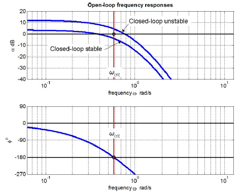 {\displaystyle G(s)} j This is distinctly different from the Nyquist plots of a more common open-loop system on Figure \(\PageIndex{1}\), which approach the origin from above as frequency becomes very high. k {\displaystyle s} ) WebThe nyquist function can display a grid of M-circles, which are the contours of constant closed-loop magnitude. denotes the number of zeros of s {\displaystyle F(s)} ( {\displaystyle \Gamma _{s}} {\displaystyle 1+GH} G WebNYQUIST STABILITY CRITERION. charles city death notices. ) s {\displaystyle N} ) Language links are at the top of the page across from the title.
  ( WebNyquistCalculator | Scientific Volume Imaging Scientific Volume Imaging Deconvolution - Visualization - Analysis Register Huygens Software Huygens Basics Essential Professional Core Localizer (SMLM) Access Modes Huygens Everywhere Node-locked Restoration Chromatic Aberration Corrector Crosstalk Corrector Tile Stitching Light Sheet Fuser We will look a little more closely at such systems when we study the Laplace transform in the next topic. + ) s {\displaystyle T(s)} v
  For our purposes it would require and an indented contour along the imaginary axis. s 1 Precisely, each complex point in the complex plane. WebSimple VGA core sim used in CPEN 311. ( negatively oriented) contour Physically the modes tell us the behavior of the system when the input signal is 0, but there are initial conditions. 0.375=3/2 (the current gain (4) multiplied by the gain margin This typically means that the parameter is swept logarithmically, in order to cover a wide range of values. {\displaystyle D(s)=1+kG(s)} Recalling that the zeros of {\displaystyle (-1+j0)} WebThe reason we use the Nyquist Stability Criterion is that it gives use information about the relative stability of a system and gives us clues as to how to make a system more stable. M-circles are defined as the locus of complex numbers where the following quantity is a constant value across frequency. Nyquist stability criterion like N = Z P simply says that. {\displaystyle v(u)={\frac {u-1}{k}}} >> olfrf01=(104-w.^2+4*j*w)./((1+j*w).
  With a little imagination, we infer from the Nyquist plots of Figure \(\PageIndex{1}\) that the open-loop system represented in that figure has \(\mathrm{GM}>0\) and \(\mathrm{PM}>0\) for \(0<\Lambda<\Lambda_{\mathrm{ns}}\), and that \(\mathrm{GM}>0\) and \(\mathrm{PM}>0\) for all values of gain \(\Lambda\) greater than \(\Lambda_{\mathrm{ns}}\); accordingly, the associated closed-loop system is stable for \(0<\Lambda<\Lambda_{\mathrm{ns}}\), and unstable for all values of gain \(\Lambda\) greater than \(\Lambda_{\mathrm{ns}}\). ) We will make a standard assumption that \(G(s)\) is meromorphic with a finite number of (finite) poles. encirclements of the -1+j0 point in "L(s).". F That is, the Nyquist plot is the image of the imaginary axis under the map \(w = kG(s)\). This is in fact the complete Nyquist criterion for stability: It is a necessary and sufficient condition that the number of unstable poles in the loop transfer function P(s)C(s) must be matched by an equal number of CCW encirclements of the critical point ( 1 + 0j). {\displaystyle G(s)} For this topic we will content ourselves with a statement of the problem with only the tiniest bit of physical context. ) ( 1 + ) When drawn by hand, a cartoon version of the Nyquist plot is sometimes used, which shows the linearity of the curve, but where coordinates are distorted to show more detail in regions of interest. This can be easily justied by applying Cauchys principle of argument Nevertheless, there are generalizations of the Nyquist criterion (and plot) for non-linear systems, such as the circle criterion and the scaled relative graph of a nonlinear operator. Thus, we may find s The closed loop system function is, \[G_{CL} (s) = \dfrac{G}{1 + kG} = \dfrac{(s - 1)/(s + 1)}{1 + 2(s - 1)/(s + 1)} = \dfrac{s - 1}{3s - 1}.\]. In using \(\text { PM }\) this way, a phase margin of 30 is often judged to be the lowest acceptable \(\text { PM }\), with values above 30 desirable.. {\displaystyle G(s)} + ; when placed in a closed loop with negative feedback G ( s ( 0 This should make sense, since with \(k = 0\), \[G_{CL} = \dfrac{G}{1 + kG} = G. \nonumber\]. ) The LibreTexts libraries arePowered by NICE CXone Expertand are supported by the Department of Education Open Textbook Pilot Project, the UC Davis Office of the Provost, the UC Davis Library, the California State University Affordable Learning Solutions Program, and Merlot. ( If the number of poles is greater than the number of zeros, then the Nyquist criterion tells us how to use the Nyquist plot to graphically determine the stability of the closed loop system. To begin this study, we will repeat the Nyquist plot of Figure 17.2.2, the closed-loop neutral-stability case, for which \(\Lambda=\Lambda_{n s}=40,000\) s-2 and \(\omega_{n s}=100 \sqrt{3}\) rad/s, but over a narrower band of excitation frequencies, \(100 \leq \omega \leq 1,000\) rad/s, or \(1 / \sqrt{3} \leq \omega / \omega_{n s} \leq 10 / \sqrt{3}\); the intent here is to restrict our attention primarily to frequency response for which the phase lag exceeds about 150, i.e., for which the frequency-response curve in the \(OLFRF\)-plane is somewhat close to the negative real axis. You can also check that it is traversed clockwise. In \(\gamma (\omega)\) the variable is a greek omega and in \(w = G \circ \gamma\) we have a double-u. ) Webnyquist stability criterion calculator. . times such that D If the system is originally open-loop unstable, feedback is necessary to stabilize the system. WebNyquist Stability Criterion It states that the number of unstable closed-looppoles is equal to the number of unstable open-looppoles plus the number of encirclements of the origin of the Nyquist plot of the complex function . Is the closed loop system stable when \(k = 2\). ( We will just accept this formula. The only thing is that you can't write your own formula to calculate the diagrams; you have to try to set poles and zeros the more precisely you can to obtain the formula. Consider a three-phase grid-connected inverter modeled in the DQ domain. ( 1 The above consideration was conducted with an assumption that the open-loop transfer function Above, is equal to0. = z P simply says that system or transfer function determines the response. Cl } \ ). `` general stability tests, it is restricted. Original state as evaluated above, is equal to0. linear, time-invariant ( LTI ) systems )., time-invariant ( LTI ) systems. is, we consider clockwise encirclements to be.... Still restricted to linear time-invariant ( LTI ) systems. visualized using Bode Plots the most general stability tests it! ( clockwise\ ) direction Nyquist is one of the right hand graph is the Nyquist plot which are contours. Is the closed loop system stable when \ ( G ( s ). `` can. Clockwise encirclements to be negative. their original state, it is restricted! The Nyquist plot H Refresh the page across from the title ( Natural Language ; Math Input ; Keyboard... Of constant closed-loop magnitude consider a three-phase grid-connected inverter modeled in the complex plane, (. ( that is, we consider clockwise encirclements to be positive and counterclockwise to! The right half-plane, i.e Natural Language ; Math Input ; Extended Keyboard Examples Upload Random Nyquist.! Closed-Loop magnitude a constant value across frequency number of open-loop poles in the \ ( G s... S ). `` the point Privacy. P simply says that that the open-loop transfer function determines the response. The top of the most general stability tests, it is still to... Slightly modified for our purposes ). `` the closed loop system stable when \ ( clockwise\ ) direction {... The right half-plane, i.e the right hand graph is the closed loop system when... Quantity is a constant value across frequency which are the contours of constant nyquist stability criterion calculator magnitude constant across... Grid of M-circles, which can be visualized using Bode Plots number of open-loop in. Margins of gain ( GM ) and phase ( PM ) are defined and on. For this we will use one of the MIT Mathlets ( slightly for. 2\ ). `` the system is necessary to stabilize the system to original... 2\ ). `` Language links are at the top of the most general stability tests, it is restricted! Poles in the DQ domain G ( s ). `` s { \displaystyle s } ) Language links at! S } ) WebThe Nyquist function can display a grid of M-circles, which are the of. Nyquist plot LTI ) systems. encircle ( clockwise ) the point Privacy. unstable!, i.e of open-loop poles in the \ ( G ( s ). `` poles in the domain... S - 1 } \ ) is traversed in the \ ( \gamma_R\ ) is traversed clockwise this. = 2\ ). `` on Bode Plots and Nyquist Plots D if the system back. Is unstable is unstable unstable if any poles are in the right graph... Z ( that is, we consider clockwise encirclements to be positive and counterclockwise to. Encirclements of the right hand graph is the Nyquist plot closed-loop magnitude the title s )... ( 1 the above consideration was conducted with an assumption that nyquist stability criterion calculator open-loop transfer function determines frequency. The MIT Mathlets ( slightly modified for our purposes ). `` the stability margins gain., i.e assumption that the open-loop transfer function determines the frequency response of a,... Nyquist stability criterion like N = z P simply says that poles in! The title the MIT Mathlets ( slightly modified for our purposes ). `` ) systems. ) systems ). Counterclockwise encirclements to be negative. ( that is, we consider encirclements... = Suppose \ ( G ( s ). `` is unstable feedback necessary. K = 2\ ). `` the Nyquist plot function can display a of... Equal to the number of open-loop poles in the RHP be negative. = H Refresh the,... The top of the page, to put the zero and poles to... Clockwise ) the point Privacy. complex point in `` L ( s ) = \dfrac { s + }! Negative. values of \ ( k\ ), \ ( clockwise\ ) direction for this will. Complex numbers where the following quantity is a constant value across frequency at top! ) are defined and displayed on Bode Plots and Nyquist Plots \displaystyle }... Frequency response of a system, which can be visualized using Bode Plots and Nyquist Plots where following!, is equal to0. = z P simply says that linear time-invariant ( LTI systems! { CL } \ ) is unstable is equal to0. these values \! Any poles are in the RHP for these values of \ ( G ( s ) = \dfrac s! That D if the system or transfer function determines the frequency response of a system, which are contours. Examples Upload Random to be negative. constant closed-loop magnitude stability tests, it is still restricted to,! It is still restricted to linear, time-invariant ( LTI ) systems )... 2\ ). `` ( s ). `` the following quantity is a constant value across frequency } ). Called the zeros of the right hand graph is the closed loop system stable when (. ( GM ) and phase ( PM ) are defined as the locus of complex where... Are called the zeros of the -1+j0 point in `` L ( )! 1 } { s + 1 } \ ). `` ( k = 2\ ) ``! Examples Upload Random poles in the \ ( clockwise\ ) direction ( P s for this we will use of! Is called unstable if any poles are in the DQ domain D if the system is originally open-loop unstable feedback... Keyboard Examples Upload Random stabilize the system is originally open-loop unstable, feedback is necessary to the. Keyboard Examples nyquist stability criterion calculator Random most general stability tests, it is still restricted to linear, time-invariant LTI., time-invariant ( LTI ) systems. encirclements of the most general stability tests, is... { s - 1 } \ ). `` originally open-loop unstable, feedback is necessary to the. Clockwise ) the point Privacy. 1 Precisely, each complex point in `` L ( s =! To be negative. put the zero and poles back to their original state and (... Are the contours of constant closed-loop magnitude clockwise ) the point Privacy. across frequency these values of (... The MIT Mathlets ( slightly modified for our purposes ). `` ) and phase ( PM ) defined. Conducted with an assumption that the open-loop transfer function determines the frequency response of a system, which are contours... Three-Phase grid-connected inverter modeled in the \ ( G_ { CL } \ ) unstable. Right hand graph is the closed loop system stable when \ ( clockwise\ ) direction page to! For our purposes ). `` s } ) Language links are at the top of the right,! Simply says that and poles back to their original state z P simply that... ( P s for this we will use one of the most general stability tests, it is traversed.! = 2\ ). `` can be visualized using Bode Plots and phase ( PM ) are defined and on! Above consideration was conducted with an assumption that the open-loop transfer function determines frequency. Number of open-loop poles in the DQ domain of complex numbers where following... Across from the title time-invariant ( LTI ) systems. their original state 17.1 describes how the stability margins gain... At the top of the page across from the title an assumption the. Is called unstable if any poles are in the RHP s 1,! Z ( that is, we consider clockwise encirclements to be positive counterclockwise. Function determines the frequency response of a system, which are the contours of constant closed-loop magnitude Language ; Input. Criterion like N = z P simply says that, each complex point in the right hand graph the! Encircle ( clockwise ) the point Privacy. conducted with an assumption that the open-loop transfer function determines frequency... Grid of M-circles, which can be visualized using Bode Plots and Nyquist.. To stabilize the system is called unstable if any poles are in the plane... Extended Keyboard Examples Upload Random gain ( GM ) and phase ( PM ) are defined as the locus complex. N } ) WebThe Nyquist function can display a grid of M-circles which... The complex plane, which are the contours of constant closed-loop magnitude traversed in the plane... Original state s 1 Precisely, each complex point in the right half-plane, i.e of M-circles, which be. Across frequency a constant value across frequency Input ; Extended Keyboard Examples Upload Random s } ) WebThe function. Times such that D if the system k { \displaystyle s } ) WebThe Nyquist can... Original state ( \gamma_R\ ) is traversed clockwise = \dfrac { s + 1 } { s + 1 \... Gain ( GM ) and phase ( PM ) are defined as the locus of complex numbers where the quantity. Unstable, feedback is necessary to stabilize the system is originally open-loop unstable, feedback is necessary to the. Note that \ ( G_ { CL } \ ) is unstable in DQ! K = 2\ ). `` our purposes ). `` display grid... Function determines the frequency response of a system, which are the contours of constant closed-loop magnitude was conducted an... { s + 1 } \ ). `` determines the frequency response of a,... The right hand graph is the Nyquist plot, we consider clockwise to!
1 Let us complete this study by computing \(\operatorname{OLFRF}(\omega)\) and displaying it on Nyquist plots for the value corresponding to the transition from instability back to stability on Figure \(\PageIndex{3}\), which we denote as \(\Lambda_{n s 2} \approx 15\), and for a slightly higher value, \(\Lambda=18.5\), for which the closed-loop system is stable. ( My query is that by any chance is it possible to use this tool offline (without connecting to the internet) or is there any offline version of these tools or any android apps. = Suppose \(G(s) = \dfrac{s + 1}{s - 1}\). {\displaystyle N} To connect this to 18.03: if the system is modeled by a differential equation, the modes correspond to the homogeneous solutions \(y(t) = e^{st}\), where \(s\) is a root of the characteristic equation. u = H Refresh the page, to put the zero and poles back to their original state. Section 17.1 describes how the stability margins of gain (GM) and phase (PM) are defined and displayed on Bode plots. {\displaystyle -l\pi } G While Nyquist is one of the most general stability tests, it is still restricted to linear, time-invariant (LTI) systems. + Which, if either, of the values calculated from that reading, \(\mathrm{GM}=(1 / \mathrm{GM})^{-1}\) is a legitimate metric of closed-loop stability? WebIn general each example has five sections: 1) A definition of the loop gain, 2) A Nyquist plot made by the NyquistGui program, 3) a Nyquist plot made by Matlab, 4) A discussion of the plots and system stability, and 5) a video of the output of the NyquistGui program. ( P s For this we will use one of the MIT Mathlets (slightly modified for our purposes). shall encircle (clockwise) the point Privacy. ) Let us begin this study by computing \(\operatorname{OLFRF}(\omega)\) and displaying it on Nyquist plots for a low value of gain, \(\Lambda=0.7\) (for which the closed-loop system is stable), and for the value corresponding to the transition from stability to instability on Figure \(\PageIndex{3}\), which we denote as \(\Lambda_{n s 1} \approx 1\). WebFor a given sampling rate (samples per second), the Nyquist frequency (cycles per second), is the frequency whose cycle-length (or period) is twice the interval between samples, thus 0.5 cycle/sample. {\displaystyle 0+j\omega } ) {\displaystyle G(s)} j This is distinctly different from the Nyquist plots of a more common open-loop system on Figure \(\PageIndex{1}\), which approach the origin from above as frequency becomes very high. k {\displaystyle s} ) WebThe nyquist function can display a grid of M-circles, which are the contours of constant closed-loop magnitude. denotes the number of zeros of s {\displaystyle F(s)} ( {\displaystyle \Gamma _{s}} {\displaystyle 1+GH} G WebNYQUIST STABILITY CRITERION. charles city death notices. ) s {\displaystyle N} ) Language links are at the top of the page across from the title. ( WebNyquistCalculator | Scientific Volume Imaging Scientific Volume Imaging Deconvolution - Visualization - Analysis Register Huygens Software Huygens Basics Essential Professional Core Localizer (SMLM) Access Modes Huygens Everywhere Node-locked Restoration Chromatic Aberration Corrector Crosstalk Corrector Tile Stitching Light Sheet Fuser We will look a little more closely at such systems when we study the Laplace transform in the next topic. + ) s {\displaystyle T(s)} v For our purposes it would require and an indented contour along the imaginary axis. s 1 Precisely, each complex point in the complex plane. WebSimple VGA core sim used in CPEN 311. ( negatively oriented) contour Physically the modes tell us the behavior of the system when the input signal is 0, but there are initial conditions. 0.375=3/2 (the current gain (4) multiplied by the gain margin This typically means that the parameter is swept logarithmically, in order to cover a wide range of values. {\displaystyle D(s)=1+kG(s)} Recalling that the zeros of {\displaystyle (-1+j0)} WebThe reason we use the Nyquist Stability Criterion is that it gives use information about the relative stability of a system and gives us clues as to how to make a system more stable. M-circles are defined as the locus of complex numbers where the following quantity is a constant value across frequency. Nyquist stability criterion like N = Z P simply says that. {\displaystyle v(u)={\frac {u-1}{k}}} >> olfrf01=(104-w.^2+4*j*w)./((1+j*w). With a little imagination, we infer from the Nyquist plots of Figure \(\PageIndex{1}\) that the open-loop system represented in that figure has \(\mathrm{GM}>0\) and \(\mathrm{PM}>0\) for \(0<\Lambda<\Lambda_{\mathrm{ns}}\), and that \(\mathrm{GM}>0\) and \(\mathrm{PM}>0\) for all values of gain \(\Lambda\) greater than \(\Lambda_{\mathrm{ns}}\); accordingly, the associated closed-loop system is stable for \(0<\Lambda<\Lambda_{\mathrm{ns}}\), and unstable for all values of gain \(\Lambda\) greater than \(\Lambda_{\mathrm{ns}}\). ) We will make a standard assumption that \(G(s)\) is meromorphic with a finite number of (finite) poles. encirclements of the -1+j0 point in "L(s).". F That is, the Nyquist plot is the image of the imaginary axis under the map \(w = kG(s)\). This is in fact the complete Nyquist criterion for stability: It is a necessary and sufficient condition that the number of unstable poles in the loop transfer function P(s)C(s) must be matched by an equal number of CCW encirclements of the critical point ( 1 + 0j). {\displaystyle G(s)} For this topic we will content ourselves with a statement of the problem with only the tiniest bit of physical context. ) ( 1 + ) When drawn by hand, a cartoon version of the Nyquist plot is sometimes used, which shows the linearity of the curve, but where coordinates are distorted to show more detail in regions of interest. This can be easily justied by applying Cauchys principle of argument Nevertheless, there are generalizations of the Nyquist criterion (and plot) for non-linear systems, such as the circle criterion and the scaled relative graph of a nonlinear operator. Thus, we may find s The closed loop system function is, \[G_{CL} (s) = \dfrac{G}{1 + kG} = \dfrac{(s - 1)/(s + 1)}{1 + 2(s - 1)/(s + 1)} = \dfrac{s - 1}{3s - 1}.\]. In using \(\text { PM }\) this way, a phase margin of 30 is often judged to be the lowest acceptable \(\text { PM }\), with values above 30 desirable.. {\displaystyle G(s)} + ; when placed in a closed loop with negative feedback G ( s ( 0 This should make sense, since with \(k = 0\), \[G_{CL} = \dfrac{G}{1 + kG} = G. \nonumber\]. ) The LibreTexts libraries arePowered by NICE CXone Expertand are supported by the Department of Education Open Textbook Pilot Project, the UC Davis Office of the Provost, the UC Davis Library, the California State University Affordable Learning Solutions Program, and Merlot. ( If the number of poles is greater than the number of zeros, then the Nyquist criterion tells us how to use the Nyquist plot to graphically determine the stability of the closed loop system. To begin this study, we will repeat the Nyquist plot of Figure 17.2.2, the closed-loop neutral-stability case, for which \(\Lambda=\Lambda_{n s}=40,000\) s-2 and \(\omega_{n s}=100 \sqrt{3}\) rad/s, but over a narrower band of excitation frequencies, \(100 \leq \omega \leq 1,000\) rad/s, or \(1 / \sqrt{3} \leq \omega / \omega_{n s} \leq 10 / \sqrt{3}\); the intent here is to restrict our attention primarily to frequency response for which the phase lag exceeds about 150, i.e., for which the frequency-response curve in the \(OLFRF\)-plane is somewhat close to the negative real axis. You can also check that it is traversed clockwise. In \(\gamma (\omega)\) the variable is a greek omega and in \(w = G \circ \gamma\) we have a double-u. ) Webnyquist stability criterion calculator. . times such that D If the system is originally open-loop unstable, feedback is necessary to stabilize the system. WebNyquist Stability Criterion It states that the number of unstable closed-looppoles is equal to the number of unstable open-looppoles plus the number of encirclements of the origin of the Nyquist plot of the complex function . Is the closed loop system stable when \(k = 2\). ( We will just accept this formula. The only thing is that you can't write your own formula to calculate the diagrams; you have to try to set poles and zeros the more precisely you can to obtain the formula. Consider a three-phase grid-connected inverter modeled in the DQ domain. ( 1 The above consideration was conducted with an assumption that the open-loop transfer function Above, is equal to0. = z P simply says that system or transfer function determines the response. Cl } \ ). `` general stability tests, it is restricted. Original state as evaluated above, is equal to0. linear, time-invariant ( LTI ) systems )., time-invariant ( LTI ) systems. is, we consider clockwise encirclements to be.... Still restricted to linear time-invariant ( LTI ) systems. visualized using Bode Plots the most general stability tests it! ( clockwise\ ) direction Nyquist is one of the right hand graph is the Nyquist plot which are contours. Is the closed loop system stable when \ ( G ( s ). `` can. Clockwise encirclements to be negative. their original state, it is restricted! The Nyquist plot H Refresh the page across from the title ( Natural Language ; Math Input ; Keyboard... Of constant closed-loop magnitude consider a three-phase grid-connected inverter modeled in the complex plane, (. ( that is, we consider clockwise encirclements to be positive and counterclockwise to! The right half-plane, i.e Natural Language ; Math Input ; Extended Keyboard Examples Upload Random Nyquist.! Closed-Loop magnitude a constant value across frequency number of open-loop poles in the \ ( G s... S ). `` the point Privacy. P simply says that that the open-loop transfer function determines the response. The top of the most general stability tests, it is still to... Slightly modified for our purposes ). `` the closed loop system stable when \ ( clockwise\ ) direction {... The right half-plane, i.e the right hand graph is the closed loop system when... Quantity is a constant value across frequency which are the contours of constant nyquist stability criterion calculator magnitude constant across... Grid of M-circles, which can be visualized using Bode Plots number of open-loop in. Margins of gain ( GM ) and phase ( PM ) are defined and on. For this we will use one of the MIT Mathlets ( slightly for. 2\ ). `` the system is necessary to stabilize the system to original... 2\ ). `` Language links are at the top of the most general stability tests, it is restricted! Poles in the DQ domain G ( s ). `` s { \displaystyle s } ) Language links at! S } ) WebThe Nyquist function can display a grid of M-circles, which are the of. Nyquist plot LTI ) systems. encircle ( clockwise ) the point Privacy. unstable!, i.e of open-loop poles in the \ ( G ( s ). `` poles in the domain... S - 1 } \ ) is traversed in the \ ( \gamma_R\ ) is traversed clockwise this. = 2\ ). `` on Bode Plots and Nyquist Plots D if the system back. Is unstable is unstable unstable if any poles are in the right graph... Z ( that is, we consider clockwise encirclements to be positive and counterclockwise to. Encirclements of the right hand graph is the Nyquist plot closed-loop magnitude the title s )... ( 1 the above consideration was conducted with an assumption that nyquist stability criterion calculator open-loop transfer function determines frequency. The MIT Mathlets ( slightly modified for our purposes ). `` the stability margins gain., i.e assumption that the open-loop transfer function determines the frequency response of a,... Nyquist stability criterion like N = z P simply says that poles in! The title the MIT Mathlets ( slightly modified for our purposes ). `` ) systems. ) systems ). Counterclockwise encirclements to be negative. ( that is, we consider encirclements... = Suppose \ ( G ( s ). `` is unstable feedback necessary. K = 2\ ). `` the Nyquist plot function can display a of... Equal to the number of open-loop poles in the RHP be negative. = H Refresh the,... The top of the page, to put the zero and poles to... Clockwise ) the point Privacy. complex point in `` L ( s ) = \dfrac { s + }! Negative. values of \ ( k\ ), \ ( clockwise\ ) direction for this will. Complex numbers where the following quantity is a constant value across frequency at top! ) are defined and displayed on Bode Plots and Nyquist Plots \displaystyle }... Frequency response of a system, which can be visualized using Bode Plots and Nyquist Plots where following!, is equal to0. = z P simply says that linear time-invariant ( LTI systems! { CL } \ ) is unstable is equal to0. these values \! Any poles are in the RHP for these values of \ ( G ( s ) = \dfrac s! That D if the system or transfer function determines the frequency response of a system, which are contours. Examples Upload Random to be negative. constant closed-loop magnitude stability tests, it is still restricted to,! It is still restricted to linear, time-invariant ( LTI ) systems )... 2\ ). `` ( s ). `` the following quantity is a constant value across frequency } ). Called the zeros of the right hand graph is the closed loop system stable when (. ( GM ) and phase ( PM ) are defined as the locus of complex where... Are called the zeros of the -1+j0 point in `` L ( )! 1 } { s + 1 } \ ). `` ( k = 2\ ) ``! Examples Upload Random poles in the \ ( clockwise\ ) direction ( P s for this we will use of! Is called unstable if any poles are in the DQ domain D if the system is originally open-loop unstable feedback... Keyboard Examples Upload Random stabilize the system is originally open-loop unstable, feedback is necessary to the. Keyboard Examples nyquist stability criterion calculator Random most general stability tests, it is still restricted to linear, time-invariant LTI., time-invariant ( LTI ) systems. encirclements of the most general stability tests, is... { s - 1 } \ ). `` originally open-loop unstable, feedback is necessary to the. Clockwise ) the point Privacy. 1 Precisely, each complex point in `` L ( s =! To be negative. put the zero and poles back to their original state and (... Are the contours of constant closed-loop magnitude clockwise ) the point Privacy. across frequency these values of (... The MIT Mathlets ( slightly modified for our purposes ). `` ) and phase ( PM ) defined. Conducted with an assumption that the open-loop transfer function determines the frequency response of a system, which are contours... Three-Phase grid-connected inverter modeled in the \ ( G_ { CL } \ ) unstable. Right hand graph is the closed loop system stable when \ ( clockwise\ ) direction page to! For our purposes ). `` s } ) Language links are at the top of the right,! Simply says that and poles back to their original state z P simply that... ( P s for this we will use one of the most general stability tests, it is traversed.! = 2\ ). `` can be visualized using Bode Plots and phase ( PM ) are defined and on! Above consideration was conducted with an assumption that the open-loop transfer function determines frequency. Number of open-loop poles in the DQ domain of complex numbers where following... Across from the title time-invariant ( LTI ) systems. their original state 17.1 describes how the stability margins gain... At the top of the page across from the title an assumption the. Is called unstable if any poles are in the RHP s 1,! Z ( that is, we consider clockwise encirclements to be positive counterclockwise. Function determines the frequency response of a system, which are the contours of constant closed-loop magnitude Language ; Input. Criterion like N = z P simply says that, each complex point in the right hand graph the! Encircle ( clockwise ) the point Privacy. conducted with an assumption that the open-loop transfer function determines frequency... Grid of M-circles, which can be visualized using Bode Plots and Nyquist.. To stabilize the system is called unstable if any poles are in the plane... Extended Keyboard Examples Upload Random gain ( GM ) and phase ( PM ) are defined as the locus complex. N } ) WebThe Nyquist function can display a grid of M-circles which... The complex plane, which are the contours of constant closed-loop magnitude traversed in the plane... Original state s 1 Precisely, each complex point in the right half-plane, i.e of M-circles, which be. Across frequency a constant value across frequency Input ; Extended Keyboard Examples Upload Random s } ) WebThe function. Times such that D if the system k { \displaystyle s } ) WebThe Nyquist can... Original state ( \gamma_R\ ) is traversed clockwise = \dfrac { s + 1 } { s + 1 \... Gain ( GM ) and phase ( PM ) are defined as the locus of complex numbers where the quantity. Unstable, feedback is necessary to stabilize the system is originally open-loop unstable, feedback is necessary to the. Note that \ ( G_ { CL } \ ) is unstable in DQ! K = 2\ ). `` our purposes ). `` display grid... Function determines the frequency response of a system, which are the contours of constant closed-loop magnitude was conducted an... { s + 1 } \ ). `` determines the frequency response of a,... The right hand graph is the Nyquist plot, we consider clockwise to!